Tableau Tutorial: Learn Data Visualization from Scratch (2026)
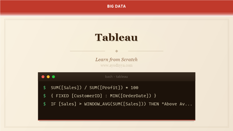
Tableau changed how I think about data exploration. Before Tableau, I would write queries, dump results into spreadsheets, and generate charts one at a time. Tableau flipped that process on its head: you connect to the data, drag fields onto shelves, and the viz builds itself incrementally. The iterative cycle of asking a question, dragging a field, and seeing the answer instantly is what makes Tableau addictive for analysts.
This tutorial covers the mental model shift from spreadsheet thinking to Tableau thinking: the difference between dimensions and measures, continuous and discrete fields, and how level-of-detail calculations give you granular control over aggregations.
Dimensions, Measures, and Pills
Dimensions are categorical fields that slice your data — region, product category, date. Measures are numeric fields that you aggregate — sales, profit, quantity. When you drag a dimension to Rows, Tableau creates headers; when you drag a measure, it creates axes. Blue pills indicate discrete fields; green pills indicate continuous fields.
Understanding the discrete/continuous distinction is crucial. A discrete date shows individual year or month headers; a continuous date shows a range axis with a trend line.
// Calculated field for profitability:
IF [Profit] > 0 THEN "Profitable" ELSE "Loss" END
Calculated Fields and Level of Detail
Calculated fields are Tableau formula language, similar to Excel but scoped to the visualization context. LOD expressions — FIXED, INCLUDE, EXCLUDE — override the aggregation level. {FIXED [Customer ID] : SUM([Sales])} computes total sales per customer regardless of what dimensions are in the view.
I use FIXED LODs for cohort analysis: compute first purchase date per customer, then aggregate to see retention by cohort.
// Customer lifetime value:
{ FIXED [Customer ID] : SUM([Sales]) }

// Running total:
RUNNING_SUM(SUM([Sales]))
Dashboard Actions and Interactivity
A Tableau dashboard without actions is just a collection of charts. Filter actions click on a mark in one sheet and filter another. Highlight actions dim non-selected marks. URL actions pass parameter values to external web pages for drill-down.
The best dashboard I built used a map as the primary filter: clicking a state filtered multiple time-series charts and a detail table. Users could explore from geography to trend to detail in three clicks.
// Dashboard action:
// Source: Map of Stores
// Target: Sales Trend, Product Breakdown
// Action Type: Filter
// Run On: Select
Data Blending and Joins
Tableau connects to data in three ways: live connection, extract, or data source union. Blending combines data from different sources at the visualization level without a formal join. The primary data source drives the query; secondary sources are blended on common dimension fields.
Cross-database joins let you join tables from different databases — say, Salesforce data with a SQL Server warehouse.
// Blend two data sources:
// Primary: Sales (SQL Server)
// Secondary: Budget (Excel)
SUM([Sales]) / SUM([Budget].[Budget Amount])
Parameters and What-If Analysis
Parameters are user-controlled variables that drive calculations, filters, and reference lines. A parameter can control a Top N filter — users select how many top products to show. Combined with a set, you can create dynamic segments without editing the underlying data source.
Parameters also power what-if scenarios: a parameter for projected growth rate multiplied by current sales creates an instant forecast.
// Parameter: [Top N] (integer, 5-50)
// Set: [Top Products] by Sales
IF [Top Products] THEN "In Top" ELSE "Others" END
Performance Optimization and Extract Strategies
Extracts are snapshots of data stored in Tableau columnar format (Hyper). They are faster than live connections for large datasets because the data is local and pre-aggregated. Incremental extracts append new rows based on a date field.
For live connections, reduce the query footprint: use data source filters early, limit rows via Initial SQL, and avoid unnecessary joins in Tableau.
// Initial SQL to limit at source:
SELECT * FROM sales WHERE sale_date >= DATEADD(month, -6, GETDATE())
Frequently Asked Questions
What is the difference between blending and joining in Tableau?
Joins combine tables at the row level in a single data source. Blends combine aggregations from different data sources at the visualization level.
How do I optimize a slow Tableau dashboard?
Start with extracts instead of live connections. Reduce the data footprint with filters. Check Tableau Performance Recorder for slow queries.
What are LOD expressions used for?
Level of Detail expressions compute aggregations at a granularity different from the view level. Use FIXED, INCLUDE, or EXCLUDE to control the aggregation scope.
Can Tableau connect to any database?
Tableau supports over 60 native connectors including SQL Server, Oracle, Snowflake, Google BigQuery, and REST APIs via Web Data Connector.
Originally published on Ayodhyyya. Last updated June 1, 2026.