Data Science and Machine Learning Tutorial from Scratch (2026)
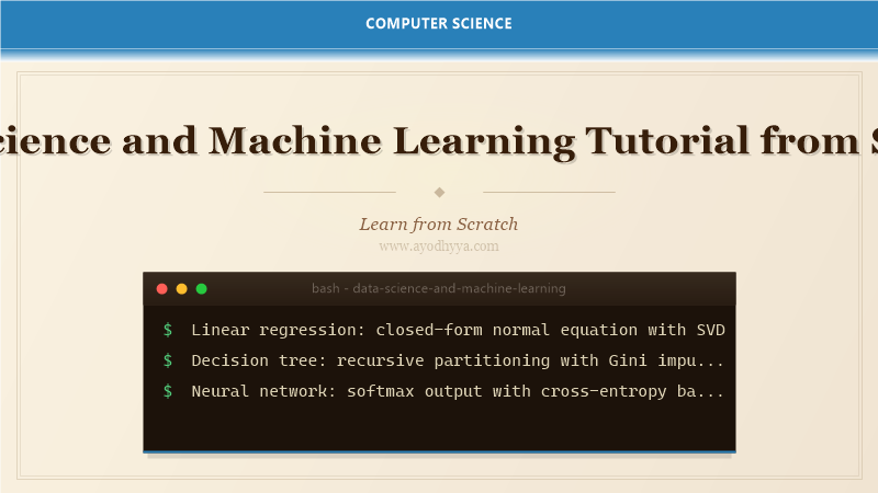
Data science combines statistics, programming, and domain expertise to extract insights from data. Machine learning enables systems to learn patterns from data without explicit programming. This tutorial covers the complete pipeline: data collection, cleaning, exploratory analysis, feature engineering, model training, evaluation, and deployment. With experience shipping ML models in production, I cover both classical algorithms and deep learning.
We will implement a regression model from scratch, build a neural network using NumPy, and deploy a model as a REST API.
Exploratory Data Analysis and Visualization
EDA is the process of understanding data through summary statistics and visualizations. Key tools: histograms (distribution), scatter plots (relationships), box plots (outliers), correlation matrices. Summary statistics: mean, median, std, min, max, quartiles. Missing data imputation includes mean/median/mode, regression imputation, or advanced methods like MICE and KNN imputation.
import numpy as np, pandas as pd
np.random.seed(42)
df = pd.DataFrame({'x': np.random.normal(0,1,100),'y': np.random.normal(0,1,100),'c': np.random.choice([0,1],100)})
print(df.describe())
print(f'Skewness: {df["x"].skew():.2f}, Kurtosis: {df["x"].kurt():.2f}')
# correlation
corr = df.corr(); print(corr)
# detect outliers - IQR
Q1,Q3 = df['x'].quantile([0.25,0.75]); IQR=Q3-Q1
outliers = df[(df['x']Q3+1.5*IQR)]
print(f'Outliers: {len(outliers)}, bounds: [{Q1-1.5*IQR:.2f},{Q3+1.5*IQR:.2f}]')
Linear Regression: From Scratch
Linear regression models y = Xw + b using the sum of squared errors loss. The closed-form solution uses the normal equation: w = (X^T X)^-1 X^T y. For numerical stability, use SVD decomposition. Gradient descent iteratively updates weights: w = w - lr * (1/m) * X^T (Xw - y). Regularization (Ridge L2, Lasso L1) prevents overfitting.
import numpy as np
class LinearRegression:
    def __init__(self, lr=0.01, epochs=1000, reg=0):
        self.lr=lr; self.epochs=epochs; self.reg=reg; self.w=None; self.b=None
    def fit(self, X, y):
        m,n=X.shape; self.w=np.zeros(n); self.b=0
        for ep in range(self.epochs):
            y_pred = X@self.w + self.b
            dw = (1/m)*X.T@(y_pred-y) + self.reg*self.w/m
            db = (1/m)*np.sum(y_pred-y)
            self.w -= self.lr*dw; self.b -= self.lr*db
            if ep%200==0: mse=np.mean((y_pred-y)**2); print(f'Ep {ep}: MSE={mse:.4f}')
    def predict(self, X): return X@self.w + self.b
    def closed_form(self, X, y):
        Xb=np.c_[np.ones(X.shape[0]),X]
        self.w=np.linalg.pinv(Xb.T@Xb)@Xb.T@y; self.b=self.w[0]; self.w=self.w[1:]
        return self
np.random.seed(42); X=np.random.randn(100,3); y=X@[2,-1,0.5]+3+np.random.randn(100)*0.1
lr=LinearRegression(lr=0.1,epochs=1000); lr.fit(X,y); print(f'Weights: {lr.w}, Bias: {lr.b:.3f}')
Logistic Regression and Classification
Logistic regression uses the sigmoid function to output probabilities: P(y=1|x) = 1/(1+exp(-z)). Decision boundary: predict 1 if P >= 0.5. Cross-entropy loss: L = -[y*log(p) + (1-y)*log(1-p)]. Gradient descent update uses the same form as linear regression (y_pred - y) because the derivative of sigmoid cancels nicely.
import numpy as np
class LogisticRegression:
    def __init__(self, lr=0.01, epochs=1000):
        self.lr=lr; self.epochs=epochs; self.w=None; self.b=None
    def sigmoid(self,z): return 1/(1+np.exp(-np.clip(z,-100,100)))
    def fit(self, X, y):
        m,n=X.shape; self.w=np.zeros(n); self.b=0
        for ep in range(self.epochs):
            z=X@self.w+self.b; p=self.sigmoid(z)
            dw=(1/m)*X.T@(p-y); db=(1/m)*np.sum(p-y)
            self.w-=self.lr*dw; self.b-=self.lr*db
            if ep%200==0:
                loss=-np.mean(y*np.log(p+1e-8)+(1-y)*np.log(1-p+1e-8))
                acc=np.mean((p>=0.5)==y); print(f'Ep {ep}: loss={loss:.4f}, acc={acc:.4f}')
    def predict(self,X,thresh=0.5): return (self.sigmoid(X@self.w+self.b)>=thresh).astype(int)
    def predict_proba(self,X): return self.sigmoid(X@self.w+self.b)
np.random.seed(42); X=np.random.randn(200,2); y=(X[:,0]+X[:,1]>0).astype(int)
logr=LogisticRegression(lr=0.1,epochs=1000); logr.fit(X,y)
Decision Trees and Ensemble Methods
Decision trees partition the feature space with recursive splits. Splits are chosen to minimize impurity: Gini impurity (CART) or entropy (ID3/C4.5). Trees overfit easily, so pruning is essential. Random Forests build multiple trees on bootstrapped samples, averaging predictions. Gradient Boosting (XGBoost, LightGBM) builds trees sequentially, each correcting residuals of the previous.
import numpy as np
class DecisionTree:
    def __init__(self, max_depth=5, min_samples=2):
        self.max_depth=max_depth; self.min_samples=min_samples; self.tree=None
    def gini(self, y):
        _,c=np.unique(y,return_counts=True); p=c/len(y); return 1-np.sum(p**2)
    def split(self, X, y):
        best=None; best_g=-float('inf')
        for f in range(X.shape[1]):
            vals=np.unique(X[:,f])
            for v in vals:
                m=X[:,f]<=v
                if np.sum(m)best_g: best_g=g; best=(f,v)
        return best
    def build(self, X, y, depth=0):
        if depth>=self.max_depth or len(np.unique(y))==1 or len(y)
Neural Networks and Deep Learning
Neural networks are universal function approximators: layers of neurons connected by weighted edges, with nonlinear activation functions (ReLU, sigmoid, tanh). Forward propagation computes outputs. Backpropagation computes gradients via the chain rule. Common architectures: MLP for tabular data, CNN for images, RNN/LSTM/Transformer for sequences. Optimization uses Adam, learning rate scheduling, batch normalization.
import numpy as np
class MLP:
    def __init__(self, layers):
        self.W=[np.random.randn(layers[i],layers[i+1])*0.01 for i in range(len(layers)-1)]
        self.b=[np.zeros((1,layers[i+1])) for i in range(len(layers)-1)]
    def relu(self,z): return np.maximum(0,z)
    def softmax(self,z): e=np.exp(z-np.max(z,axis=1,keepdims=True)); return e/np.sum(e,axis=1,keepdims=True)
    def forward(self, X):
        a=X; self.zs=[]; self.as_=[X]
        for i in range(len(self.W)-1):
            z=a@self.W[i]+self.b[i]; self.zs.append(z); a=self.relu(z); self.as_.append(a)
        z=a@self.W[-1]+self.b[-1]; self.zs.append(z); a=self.softmax(z); self.as_.append(a)
        return a
    def backward(self, X, y, lr=0.01):
        m=X.shape[0]; y_one_hot=np.eye(self.as_[-1].shape[1])[y]
        da=self.as_[-1]-y_one_hot
        for i in reversed(range(len(self.W))):
            dz=da; dw=self.as_[i].T@dz/m; db=np.sum(dz,axis=0,keepdims=True)/m
            if i>0: da=dz@self.W[i].T*(self.as_[i]>0)
            self.W[i]-=lr*dw; self.b[i]-=lr*db
    def train(self,X,y,epochs=100,lr=0.01):
        for ep in range(epochs): pred=self.forward(X); loss=-np.mean(np.log(pred[np.arange(len(y)),y]+1e-8)); self.backward(X,y,lr)
            if ep%20==0: print(f'Epoch {ep}, loss={loss:.4f}, acc={np.mean(np.argmax(pred,1)==y):.4f}')
MLOps: Model Deployment and Monitoring
MLOps operationalizes ML models. Key components: feature store (centralized feature computation), model registry (versioned model storage), serving infrastructure (REST/gRPC endpoints, batch inference), monitoring (data drift, model drift, prediction latency), and retraining pipelines. A/B testing and canary deployments validate model performance in production.
from flask import Flask, request, jsonify
import joblib
app=Flask(__name__); model=joblib.load('model.pkl')
class FeatureStore:
    def __init__(self): self.feats={}
    def compute(self, key, fns):
        if key not in self.feats:
            self.feats[key]={name:fn() for name,fn in fns.items()}
        return self.feats[key]
class ModelMonitor:
    def __init__(self, ref): self.ref=ref; self.preds=[]; self.drift_thresh=0.1
    def log(self, X, y_pred, y_true=None):
        self.preds.append({'X':X,'y_pred':y_pred,'y_true':y_true,'ts':__import__('time').time()})
    def detect_drift(self):
        if len(self.preds)<100: return False
        recent=[p['y_pred'] for p in self.preds[-100:]]
        drift=abs(np.mean(recent)-np.mean(self.ref))
        return drift>self.drift_thresh, drift
@app.route('/predict',methods=['POST'])
def predict(): data=request.json; pred=model.predict([data['feats']])[0]; return jsonify({'prediction':int(pred),'prob':float(max(model.predict_proba([data['feats']])[0]))})
Frequently Asked Questions
What is the difference between supervised and unsupervised learning?
Supervised learning uses labeled data (X,y) to learn a mapping. Unsupervised learning finds patterns in unlabeled data (X only), like clustering or dimensionality reduction.
What is overfitting and how to prevent it?
Overfitting occurs when the model learns noise instead of signal. Prevention: regularization (L1/L2), cross-validation, early stopping, more training data, simpler models.
What is the bias-variance tradeoff?
Bias is error from overly simplistic assumptions. Variance is error from sensitivity to training data. Complex models have low bias, high variance. Simple models have high bias, low variance.
What is gradient descent and why does it work?
Gradient descent moves parameters in the direction of steepest descent of the loss function. It works because the negative gradient points toward the local minimum for convex functions.
Originally published on Ayodhyyya. Last updated June 1, 2026.