Data Structures Tutorial: Learn DSA from Scratch (2026)
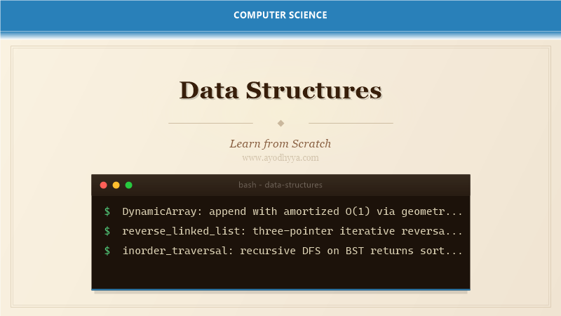
Data structures are the bedrock of efficient software — every program you write spends its life organizing and manipulating data. Over years of building systems at scale, I have learned that choosing the right data structure is often the difference between a responsive application and one that buckles under load. This tutorial distills that hard-won experience into a practical guide, from primitive arrays to advanced tries and graphs, with an emphasis on real-world trade-offs.
We will explore how each structure organizes memory, what operations it accelerates, and where it falls short. The goal is not just to memorize definitions but to develop an intuition for when a hash table outperforms a binary search tree, or why a linked list might be the right choice despite its cache-unfriendly layout.
Arrays and Dynamic Arrays
Arrays are the simplest and most widely used data structure. They store elements in contiguous memory locations, providing O(1) random access by index. The catch is that insertion and deletion at arbitrary positions require shifting elements, yielding O(n) cost. Dynamic arrays — like Python's list or C++'s std::vector — amortize resizing by allocating extra capacity, so appending remains O(1) on average. When the underlying block fills up, a new block (typically 2x larger) is allocated and elements are copied over.
# Dynamic array append with amortized analysis
class DynamicArray:
    def __init__(self):
        self.capacity = 1
        self.data = [None] * self.capacity
        self.size = 0

    def append(self, value):
        if self.size == self.capacity:
            self.capacity *= 2
            new_data = [None] * self.capacity
            for i in range(self.size):
                new_data[i] = self.data[i]
            self.data = new_data
        self.data[self.size] = value
        self.size += 1
Linked Lists
Linked lists sacrifice random access for O(1) insertions and deletions at known positions. Each node stores a value and a pointer to the next node (singly linked) or both next and previous (doubly linked). In practice, linked lists are rarely the default choice because of poor cache locality — each node may be scattered across heap memory. However, they shine in scenarios like implementing undo/redo stacks, adjacency lists for sparse graphs, or lock-free concurrent queues using CAS primitives.
class ListNode:
    def __init__(self, val=0, next=None):
        self.val = val
        self.next = next

def reverse_linked_list(head):
    prev = None
    curr = head
    while curr:
        nxt = curr.next
        curr.next = prev
        prev = curr
        curr = nxt
    return prev
Stacks and Queues
Stacks follow Last-In-First-Out (LIFO) order, while queues follow First-In-First-Out (FIFO). These are not just theoretical constructs — a stack powers the call stack in every programming language, and a queue manages task scheduling in operating systems. Circular queues reuse array space efficiently by wrapping the tail index around. Deques (double-ended queues) support O(1) insertion and removal at both ends, making them versatile for sliding window problems.
class Queue:
    def __init__(self, capacity):
        self.capacity = capacity
        self.buffer = [None] * capacity
        self.head = 0
        self.tail = 0
        self.count = 0

    def enqueue(self, item):
        if self.count == self.capacity:
            raise OverflowError
        self.buffer[self.tail] = item
        self.tail = (self.tail + 1) % self.capacity
        self.count += 1

    def dequeue(self):
        if self.count == 0:
            return None
        item = self.buffer[self.head]
        self.head = (self.head + 1) % self.capacity
        self.count -= 1
        return item
Hash Tables
Hash tables map keys to values using a hash function and provide average O(1) lookups. Collisions are inevitable — two common resolution strategies are chaining (linked list per bucket) and open addressing (probing for the next free slot). A well-designed hash function minimizes collisions, but resizing and rehashing are necessary as the load factor grows. Practical refinements include Robin Hood hashing, which reduces probe variance, and Cuckoo hashing, which guarantees O(1) worst-case lookup.
class HashTable:
    def __init__(self, capacity=16):
        self.capacity = capacity
        self.buckets = [[] for _ in range(capacity)]

    def _hash(self, key):
        return hash(key) % self.capacity

    def put(self, key, value):
        idx = self._hash(key)
        for i, (k, v) in enumerate(self.buckets[idx]):
            if k == key:
                self.buckets[idx][i] = (key, value)
                return
        self.buckets[idx].append((key, value))
Trees and Binary Search Trees
Trees represent hierarchical relationships — file systems, DOM structures, and parse trees all map to tree data structures. A binary search tree maintains the invariant that all nodes in the left subtree are smaller than the root, and all in the right subtree are larger. This yields O(log n) search in the balanced case, but degenerates to O(n) if inserts arrive in sorted order. Self-balancing variants like AVL trees and Red-Black trees enforce height bounds through rotations and color flips.
class TreeNode:
    def __init__(self, val):
        self.val = val
        self.left = None
        self.right = None

def inorder_traversal(node):
    if node is None:
        return []
    return inorder_traversal(node.left) + [node.val] + inorder_traversal(node.right)
Graphs: Adjacency Lists and Traversals
Graphs model pairwise relationships — social networks, road maps, and dependency graphs. Adjacency lists store for each vertex a list of its neighbors, consuming O(V + E) space and enabling efficient iteration over edges. Two fundamental traversals are Depth-First Search (DFS), which explores as far as possible before backtracking, and Breadth-First Search (BFS), which explores level by level. BFS finds the shortest path in unweighted graphs, while DFS is useful for topological sorting and detecting cycles.
from collections import deque

def bfs(graph, start):
    visited = set()
    queue = deque([start])
    order = []
    while queue:
        node = queue.popleft()
        if node not in visited:
            visited.add(node)
            order.append(node)
            for neighbor in graph[node]:
                if neighbor not in visited:
                    queue.append(neighbor)
    return order
Frequently Asked Questions
What data structure should I use for fast lookups by key?
A hash table provides average O(1) lookups, insertions, and deletions. Use it when order does not matter. If you need sorted key traversal, prefer a balanced BST (e.g., TreeMap in Java) or a skip list.
Why are linked lists less performant than arrays in practice?
Linked list nodes are scattered across heap memory, causing poor cache locality. Modern CPUs are heavily optimized for sequential memory access (prefetching), so arrays often outperform linked lists even when algorithmic complexity suggests otherwise.
When would I use a trie over a hash table?
Tries excel for prefix-based searches, autocomplete, and dictionary word validation. They are more memory-efficient for keys sharing common prefixes, and they support ordered iteration. However, they are slower for exact key lookups compared to hash tables.
What is the difference between a stack and a heap data structure?
A stack is a LIFO structure used for function call management and local variables; memory is automatically reclaimed. A heap (not to be confused with the memory heap) is a tree-based structure for priority queues, supporting O(log n) insertion and extraction of the min or max element.
Originally published on Ayodhyyya. Last updated June 1, 2026.