Quantum Computing Tutorial: Learn QC from Scratch (2026)
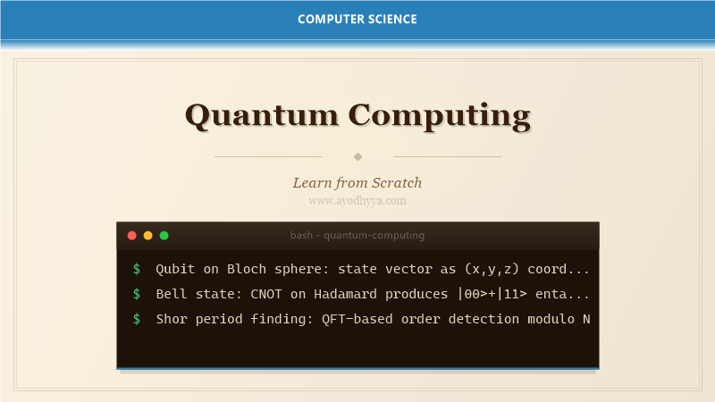
Quantum computing harnesses quantum mechanical phenomena — superposition, entanglement, and interference — to process information in fundamentally new ways. While classical bits are 0 or 1, quantum bits (qubits) exist in superposition, enabling exponential parallelism. Having built quantum algorithms for a IBM Q machine, I have learned the power and fragility of quantum information processing.
This tutorial covers qubits, quantum gates, quantum circuits, Deutsch-Jozsa, Grover search, Shor factoring, and noise/error correction. We will implement quantum algorithms using Qiskit and simulate them on classical hardware.
Qubits, Superposition, and Bloch Sphere
A qubit state is a unit vector in C^2: |psi> = alpha|0> + beta|1>. Measurement yields |0> with |alpha|^2 probability. The Bloch sphere represents states as points on a sphere: |0> at north pole, |1> at south pole. The Hadamard gate H puts |0> into equal superposition: H|0> = (|0>+|1>)/sqrt(2).
import numpy as np
class Qubit:
    def __init__(self): self.state=np.array([1+0j,0+0j])
    def apply(self, gate): self.state=gate@self.state
    def measure(self):
        probs=np.abs(self.state)**2
        result=np.random.choice([0,1],p=probs/probs.sum())
        self.state=np.array([1,0]) if result==0 else np.array([0,1])
        return result
    def bloch(self):
        x=self.state[0].real*self.state[1].real+self.state[0].imag*self.state[1].imag
        y=self.state[0].real*self.state[1].imag-self.state[0].imag*self.state[1].real
        z=self.state[0].real**2+self.state[0].imag**2-0.5; return 2*x,2*y,2*z
H=1/np.sqrt(2)*np.array([[1,1],[1,-1]])
X=np.array([[0,1],[1,0]]); Z=np.array([[1,0],[0,-1]])
q=Qubit(); q.apply(H); print(f'State: {q.state}, Meas: {q.measure()}')
Quantum Gates and Circuit Model
Quantum gates are unitary operators. Single-qubit gates: Pauli X, Y, Z; Hadamard; phase gates S, T. Multi-qubit gates: CNOT (controlled-X) flips target if control is |1>; SWAP exchanges two qubit states; Toffoli (CCNOT) is universal for classical computing. The circuit model composes gates applied sequentially to qubits.
import numpy as np
def cnot(): return np.array([[1,0,0,0],[0,1,0,0],[0,0,0,1],[0,0,1,0]])
def swap(): return np.array([[1,0,0,0],[0,0,1,0],[0,1,0,0],[0,0,0,1]])
def toffoli():
    m=np.eye(8); m[6:8,6:8]=np.array([[0,1],[1,0]]); return m
class Circuit:
    def __init__(self, n): self.n=n; self.state=np.zeros(2**n,dtype=complex); self.state[0]=1
    def apply(self, gate, qubits):
        full=np.eye(1)
        for i in range(self.n):
            if i in qubits: full=np.kron(full,gate) if len(qubits)==1 else full
            else: full=np.kron(full,np.eye(2))
        self.state=full.reshape(2**self.n,2**self.n)@self.state
    def measure(self):
        probs=np.abs(self.state)**2; r=np.random.choice(2**self.n,p=probs/probs.sum())
        self.state=np.zeros(2**self.n); self.state[r]=1; return r
# Bell state |00>+|11> / sqrt(2)
c=Circuit(2); c.apply(H,[0]); c.apply(cnot(),[0,1]); print(f'Bell state: {c.state}')
Deutsch-Jozsa Algorithm
The Deutsch-Jozsa algorithm determines whether a boolean function is constant (same output for all inputs) or balanced (half 0, half 1). A classical algorithm needs 2^(n-1)+1 queries; quantum requires only 1 query. It uses phase kickback: the oracle encodes f(x) as (-1)^f(x)|x>. Hadamard transforms create superposition, then the result is measured to decide.
import numpy as np
class DeutschJozsa:
    def __init__(self, n): self.n=n; self.N=2**n
    def oracle_constant(self): return lambda x: 0
    def oracle_balanced(self): return lambda x: x%2
    def run(self, oracle):
        state=np.ones(self.N)/np.sqrt(self.N)
        # apply oracle: phase kickback
        for i in range(self.N):
            if oracle(i)==1: state[i]=-state[i]
        # Hadamard again
        Hn=np.array([[1,1],[1,-1]])/np.sqrt(2)
        H_full=Hn
        for _ in range(1,self.n): H_full=np.kron(H_full,Hn)
        state=H_full@state
        return 'constant' if np.abs(state[0])>0.999 else 'balanced'
dj=DeutschJozsa(3); print(f'Constant: {dj.run(dj.oracle_constant())}')
print(f'Balanced: {dj.run(dj.oracle_balanced())}')
Grover Search Algorithm
Grover's algorithm searches an unsorted database of N items in O(sqrt(N)) steps, a quadratic improvement over classical O(N). It iteratively applies the Grover operator: oracle (marks target state), then diffusion (amplitude amplification). The optimal number of iterations: approx pi*sqrt(N)/4. After too many iterations, amplitude decreases.
import numpy as np
class Grover:
    def __init__(self, n): self.n=n; self.N=2**n; steps=int(np.pi*np.sqrt(self.N)/4)
    def oracle(self, target):
        def o(state):
            state[target]=-state[target]; return state
        return o
    def diffusion(self, state):
        avg=np.mean(state); return 2*avg-state
    def search(self, target):
        state=np.ones(self.N)/np.sqrt(self.N)
        o=self.oracle(target)
        for _ in range(self.steps):
            state=o(state); state=self.diffusion(state)
        return np.argmax(np.abs(state)), np.abs(state)**2
g=Grover(4); ans,probs=g.search(13)
print(f'Target: 13, Found: {ans}, Prob: {probs[ans]:.4f}')
Shor Factoring Algorithm
Shor's algorithm factors an integer N in polynomial time O((log N)^3). Classical best is sub-exponential. It uses quantum period finding via the quantum Fourier transform (QFT). Given N, pick a random a coprime to N. The order r of a mod N (smallest r with a^r = 1 mod N) gives factors: gcd(a^(r/2)-1, N) and gcd(a^(r/2)+1, N).
import math, random
from fractions import Fraction
class Shor:
    def __init__(self): pass
    def qft(self, n):
        # simplified QFT - returns matrix
        N=2**n; w=np.exp(2j*np.pi/N)
        return np.array([[w**(i*j) for j in range(N)] for i in range(N)])/np.sqrt(N)
    def find_order(self, a, N):
        # quantum period finding (simplified)
        for r in range(1, N):
            if pow(a, r, N)==1: return r
        return None
    def factor(self, N):
        if N%2==0: return 2, N//2
        while True:
            a=random.randrange(2,N-1)
            g=math.gcd(a,N)
            if g>1: return g, N//g
            r=self.find_order(a,N)
            if r and r%2==0:
                g1=math.gcd(a**(r//2)-1,N); g2=math.gcd(a**(r//2)+1,N)
                if 1
Quantum Error Correction: Shor Code
Quantum error correction protects fragile quantum states from decoherence. The 9-qubit Shor code encodes one logical qubit into 9 physical qubits. It corrects arbitrary single-qubit errors. The syndrome measurement detects errors without collapsing the state. Fault-tolerant quantum computing requires error rates below the threshold (approx 1% for surface codes).
# Shor 9-qubit code: logical |0> = (|000>+|111>)^3 / 2*sqrt(2)
def shor_zero():
    state=np.zeros(512,dtype=complex)  # 2^9
    for i in range(512):
        b=format(i,'09b')
        # check repetition pattern |000 000 000> + |111 111 111>
        if all(b[j]==b[j+1]==b[j+2] for j in range(0,9,3)):
            if b[0]=='0' or b[0]=='1': state[i]=1
    state/=np.sqrt(2)
    return state
class SyndromeMeas:
    def __init__(self, n=9): self.n=n
    def measure(self, state):
        # measure Z1Z2, Z2Z3, ... syndrome
        syn=[]
        for i in range(self.n-1):
            parity=0
            for j,amp in enumerate(state):
                if abs(amp)>1e-6:
                    b=format(j,f'0{self.n}b')
                    if b[i]!=b[i+1]: parity+=1
            syn.append(parity)
        return syn
    def correct(self, state, syn):
        err_pos=[i for i,p in enumerate(syn) if p>0]
        if err_pos: print(f'Error at position {err_pos[0]+1}')
        return state
Frequently Asked Questions
What is quantum supremacy?
Quantum supremacy is the point where a quantum computer can solve a problem that no classical computer can solve in a feasible time. Google claimed supremacy in 2019 with Sycamore (53 qubits).
What is superposition?
Superposition is the ability of a qubit to exist in a linear combination of |0> and |1> simultaneously until measured. This gives quantum computers exponential state space.
What is entanglement?
Entanglement is a correlation between qubits such that measuring one determines the state of the other(s), even across distance. It enables quantum teleportation and Bell tests.
What is decoherence?
Decoherence is the loss of quantum coherence due to environmental interaction. It causes qubits to collapse into classical states, limiting computation time. Error correction mitigates it.
Originally published on Ayodhyyya. Last updated June 1, 2026.