Getting Started with Cassandra

Apache Cassandra is a distributed NoSQL database designed for high availability and linear scalability. There is no single point of failure. Data is automatically replicated across multiple nodes and multiple data centers. Cassandra is built for write-heavy workloads: time-series data, IoT sensor readings, event logging, messaging systems, and recommendation engines.

Installation starts with Java 8 or 11. Download the binary from the Apache site or use a package manager. Extract the tarball, configure cassandra.yaml with your cluster name and seeds, and run bin/cassandra. The default configuration works for a single-node test cluster. Connect with cqlsh, the Cassandra Query Language shell, which uses a SQL-like syntax.

# Start Cassandra
bin/cassandra

# Connect with cqlsh
cqlsh 127.0.0.1 9042

-- Create keyspace (similar to a database)
CREATE KEYSPACE myapp
WITH replication = {
    'class': 'SimpleStrategy',
    'replication_factor': 1
};

USE myapp;

CREATE TABLE users (
    user_id UUID PRIMARY KEY,
    name TEXT,
    email TEXT,
    created_at TIMESTAMP
);

Data Modeling with Query-First Design

Cassandra data modeling inverts the relational approach. In a relational database, you normalize data and use JOINs at query time. In Cassandra, you design tables for specific queries. Each query gets its own table. Data is duplicated across tables, and you accept storage redundancy for query performance. This is not wasteful, it is intentional.

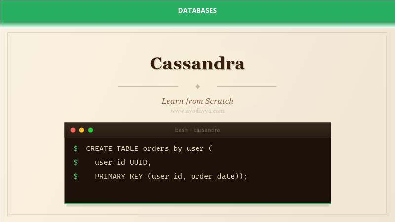
The primary key determines how data is distributed and stored. The partition key (the first part of the primary key) determines which node stores the data. Clustering columns determine the sort order within a partition. To model a query like find all orders for a customer sorted by date, use PRIMARY KEY (customer_id, order_date). All orders for a customer are stored together and sorted by date.

Avoid using wide partitions. A partition that stores millions of rows becomes a hot spot. Keep partitions under 100MB. If a customer could have millions of orders, use a composite partition key like (customer_id, year) to split data across partitions. The query becomes filtering by customer and year, which is still efficient.

-- Query-first design
-- Query: Get recent orders by user
CREATE TABLE orders_by_user (
    user_id UUID,
    order_date DATE,
    order_id UUID,
    total DECIMAL,
    status TEXT,
    PRIMARY KEY (user_id, order_date, order_id)
) WITH CLUSTERING ORDER BY (order_date DESC, order_id ASC);

CQL: Cassandra Query Language in Practice

CQL looks similar to SQL but has important differences. SELECT statements must include the partition key in the WHERE clause unless you use ALLOW FILTERING, which performs a full cluster scan. You can only filter on clustering columns within a partition. You cannot use JOINs, subqueries, or GROUP BY in the traditional sense.

INSERT and UPDATE are equivalent in Cassandra. If you INSERT a row that already exists, it counts as an upsert. There is no read-before-write, which makes writes incredibly fast. Use UPDATE for explicit timestamp control or lightweight transactions (IF conditions). Cassandra uses timestamps to resolve conflicts: the last write wins based on client-provided timestamps.

TTL (Time-To-Live) is a first-class feature. Set TTL on INSERT or UPDATE to auto-expire data. This is perfect for session data, temporary tokens, and time-series data with a retention period. Expired data is automatically deleted during compaction, but you can also read it before compaction completes. Cassandra does not delete the data instantly, it marks it with a tombstone.

-- CQL query patterns
-- Must include partition key
SELECT * FROM orders_by_user
WHERE user_id = 123e4567-e89b-12d3-a456-426614174000
  AND order_date >= '2026-01-01';

-- Upsert with TTL
INSERT INTO sessions (session_id, user_data, expires)
VALUES ('abc123', '{"role": "admin"}', toTimestamp(now()))
USING TTL 86400;

-- Counter table
CREATE TABLE page_views (
    page_id TEXT PRIMARY KEY,
    view_count COUNTER
);

UPDATE page_views SET view_count = view_count + 1
WHERE page_id = '/home';

Architecture: Gossip, Snitch, and Ring

Cassandra uses a peer-to-peer architecture with no master node. Every node is identical and communicates using the Gossip protocol. Gossip ensures that each node knows about all other nodes, their status, and their token ranges. A new node announces itself through gossip, and within seconds the entire cluster knows about it.

The snitch determines the relative proximity of nodes in the network. It tells Cassandra which nodes are in the same rack or data center. The network topology strategy for replication places replicas on different racks to tolerate rack failures and on different data centers for disaster recovery. Use the GossipingPropertyFileSnitch for production: it uses a configuration file to map IP addresses to data centers and racks.

The partitioner determines how data is distributed across the cluster. The default Murmur3Partitioner uses a hash of the partition key to assign data to one of the 2^64 token ranges. Each node owns a contiguous range of tokens. When you add a node, it takes over a portion of each existing node's token range, and data streams to the new node automatically.

-- Check cluster information
SELECT peer, data_center, rack, schema_version
FROM system.peers;

-- Check token ranges per node
SELECT peer, tokens
FROM system.peers;

-- nodetool commands
# nodetool status
# nodetool info
# nodetool ring
# nodetool gossipinfo

Consistency Levels and Tunable Consistency

Cassandra provides tunable consistency, letting you choose the trade-off between consistency and availability for each query. The consistency level determines how many replicas must respond for a read or write to succeed. ONE responds after one replica, QUORUM requires a majority, and ALL requires every replica. Weaker consistency gives lower latency and higher availability.

For writes, the client sends the write to a coordinator node, which forwards it to all replicas based on the replication factor. With CL.ONE, the coordinator acknowledges after the first replica writes. With CL.QUORUM, it waits for a majority. Hinted handoff means other replicas receive the write when they come back online.

Read repair is a background process that fixes inconsistent data during read operations. When a read uses CL.QUORUM, Cassandra compares data from all responding replicas. If any replica has stale data, it returns the latest to the client and initiates a read repair to update stale replicas. This means eventual consistency with read repair converges over time.

// Java driver with consistency levels
Cluster cluster = Cluster.builder()
    .addContactPoint("127.0.0.1")
    .build();

Session session = cluster.connect();

// Strong consistency
Statement write = new SimpleStatement(
    "INSERT INTO orders (id, status) VALUES (?, ?)",
    orderId, "shipped"
);
write.setConsistencyLevel(ConsistencyLevel.QUORUM);
session.execute(write);

// Eventual consistency for read
Statement read = new SimpleStatement(
    "SELECT * FROM orders WHERE id = ?", orderId
);
read.setConsistencyLevel(ConsistencyLevel.ONE);
session.execute(read);

Operations: Compaction, Repair, and Monitoring

Cassandra stores data in SSTables (Sorted String Tables) on disk. SSTables are immutable: once written, they never change. Writes go to a MemTable in memory and are flushed to an SSTable when full. Over time, multiple SSTables accumulate for the same partition, and reads must merge them. Compaction merges SSTables, removes tombstones and expired data, and creates new consolidated SSTables.

There are several compaction strategies. SizeTieredCompactionStrategy (STCS) merges SSTables of similar size. It is simple but can cause read amplification. LeveledCompactionStrategy (LCS) organizes SSTables into levels, keeping data in smaller, more uniform SSTables with better read performance. TimeWindowCompactionStrategy (TWCS) is designed for time-series data, compacting within defined time windows.

Repair ensures data consistency across replicas. The incremental repair process compares Merkle trees of data across replicas and streams differences. Run nodetool repair weekly to prevent data drift. Monitor key metrics in nodetool tablestats: pending compactions, read/write latency percentiles, and dropped mutations. OpsCenter provides a graphical dashboard, but I prefer Prometheus and Grafana with the Cassandra exporter.

# nodetool operations
# Force compaction
nodetool compact myapp

# Run incremental repair
nodetool repair --incremental myapp

# Check table statistics
nodetool tablestats myapp.orders_by_user

# Clean up after removing a node
nodetool cleanup myapp