Reinforcement Learning Tutorial: From Q-Learning to PPO (2026)
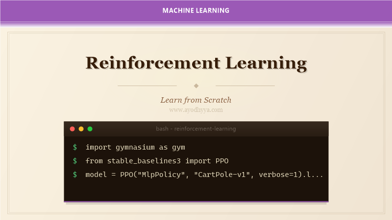
RL trains agents to make sequences of decisions through trial and error, balancing exploration and exploitation. This paradigm has produced breakthroughs in game playing and robotics.
By 2026, RL has matured with Gymnasium environments and Stable-Baselines3 providing production-ready implementations of standard algorithms.
Gymnasium Environment Setup
Gymnasium provides a standard RL interface with reset(), step(), observation space, and action space. Classic control environments like CartPole are fast to simulate.
I recommend starting with CartPole, MountainCar, and LunarLander for their clear learning signals.
import gymnasium as gym\nenv = gym.make("CartPole-v1")\nobs, info = env.reset()\nfor step in range(200):\n action = env.action_space.sample()\n obs, reward, terminated, truncated, info = env.step(action)Q-Learning Fundamentals
Q-Learning learns expected future rewards stored in a Q-table using epsilon-greedy exploration and the Bellman equation update rule.
Tabular Q-Learning works well for small discrete state spaces like Taxi-v3. Optimal performance within 500 episodes with learning rate 0.1.
q_table = np.zeros((state_space_size, action_space_size))\ndef epsilon_greedy(state, epsilon):\n return np.argmax(q_table[state]) if np.random.random() >= epsilon else env.action_space.sample()Deep Q-Networks
DQN extends Q-Learning to high-dimensional states using neural networks, experience replay, and target networks. Without these, training diverges.
A replay buffer of 100,000 transitions with target network updates every 1,000 steps worked well across Atari environments.
batch = replay_buffer.sample(batch_size)\ncurrent_q = online_network(states).gather(1, actions)\nnext_q = target_network(next_states).max(1)[0]\ntarget_q = rewards + gamma * next_q * (1 - dones)Policy Gradient Methods
Policy gradients optimize the policy directly. Actor-Critic combines policy learning with value function approximation to reduce variance.
Switching from REINFORCE to A2C on a continuous control task made training stable and converged in half the episodes.
log_probs = torch.log(actor(state).gather(1, actions))\nadvantage = returns - critic(state).detach()\nactor_loss = -(log_probs * advantage).mean()Proximal Policy Optimization
PPO clips the probability ratio between new and old policies for stable updates. It combines sample efficiency with trust-region stability.
PPO is my first-choice algorithm for any new RL problem. The SB3 implementation handles GAE, orthogonal initialization, and reward normalization.
from stable_baselines3 import PPO\nmodel = PPO("MlpPolicy", "CartPole-v1", learning_rate=3e-4, n_steps=2048, clip_range=0.2)\nmodel.learn(total_timesteps=100_000)Reward Shaping and Curriculum Learning
Sparse rewards make learning extremely difficult. Reward shaping adds intermediate guidance. Curriculum learning starts easy and increases difficulty.
Curriculum learning reduced training time for a robotic reaching task from 10 million to 2 million steps.
def shaped_reward(state, next_state):\n return raw_reward - 0.1 * np.linalg.norm(next_state - target)\ndef get_curriculum_level(episode):\n return min(episode // 1000, 5)Frequently Asked Questions
On-policy vs off-policy?
On-policy (PPO, A2C) learns from current policy data. Off-policy (DQN, SAC) reuses any data. Off-policy is more sample-efficient but less stable.
How many episodes needed?
CartPole: 100-500 episodes. Atari: 1-10 million steps. Robotics: 10-100 million steps. Use TensorBoard to track progress.
What is exploration-exploitation tradeoff?
Exploration tries new actions, exploitation uses known good actions. Managed through epsilon decay, entropy bonuses, or noise injection.
SB3 or implement from scratch?
Use SB3 for production and research baselines. Implement from scratch only for education or when modifying algorithms.
Originally published on Ayodhyyya. Last updated June 1, 2026.