R Tutorial: Learn Statistical Computing from Scratch (2026)
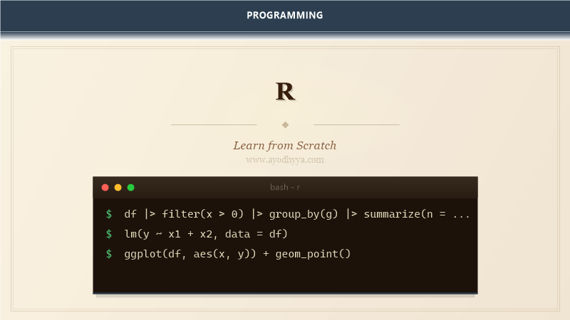
R is the language of choice for statistical analysis and data visualization, and after years of using it for data science projects, I understand why. Its vectorized operations, rich package ecosystem (CRAN hosts over 20,000 packages), and unmatched visualization capabilities make it indispensable for anyone working with data.
This tutorial covers the tools I actually use daily: data wrangling with the tidyverse, visualization with ggplot2, and statistical modeling. R is not the fastest language, but for interactive data exploration, nothing beats it.
Tidyverse
The tidyverse is a collection of packages for data science that share a common philosophy: tidyr for reshaping, dplyr for transformation, and readr for importing. Pipes (%>% or |>) chain operations sequentially. Functions like filter(), select(), mutate(), and summarize() replace base R's inconsistent syntax.
library(tidyverse)

df <- read_csv("data.csv")

result <- df |>
  filter(age >= 18) |>
  group_by(city) |>
  summarize(
    avg_income = mean(income, na.rm = TRUE),
    count = n()
  ) |>
  arrange(desc(avg_income))
ggplot2
ggplot2 implements the Grammar of Graphics: every plot is built from data, aesthetic mappings, geometric objects, and coordinate systems. Start with ggplot(data, aes(x, y)), add layers with + geom_point(), and refine with scales, themes, and facets. Once you internalize the grammar, creating publication-quality figures becomes fast and intuitive.
library(ggplot2)

ggplot(mtcars, aes(x = wt, y = mpg)) +
  geom_point(aes(color = factor(cyl)), size = 3) +
  geom_smooth(method = "lm", se = FALSE) +
  labs(
    title = "MPG vs Weight",
    x = "Weight (1000 lbs)",
    y = "Miles per Gallon"
  ) +
  theme_minimal()
Data.table
data.table is optimized for speed and memory efficiency on large datasets. Its syntax DT[i, j, by] reads as: filter rows (i), compute columns (j), group by (by). For datasets with millions of rows, data.table outperforms dplyr significantly. Use setkey() for fast binary search joins.
library(data.table)

dt <- fread("large_data.csv")
setkey(dt, user_id)

result <- dt[
  age > 18,
  .(avg = mean(score), total = .N),
  by = .(city)
][order(-avg)]

# Fast join
other <- data.table(user_id = 1:1000, status = "active")
merged <- dt[other, on = "user_id"]
Statistical Models
R's native modeling syntax y ~ x1 + x2 is concise and consistent across model types. lm() fits linear models; glm() fits generalized linear models; lmer() from lme4 fits mixed effects. The summary() function provides coefficients, p-values, and fit statistics. Plot diagnostics with plot(model).
model <- lm(mpg ~ wt + factor(cyl), data = mtcars)
summary(model)

# Predictions
new_cars <- data.frame(wt = c(2.5, 3.0), cyl = c(4, 6))
predictions <- predict(model, newdata = new_cars,
                       interval = "confidence")
print(predictions)
R Markdown
R Markdown combines narrative text, code, and results in a single document. Code chunks execute when you knit the document, and results (tables, plots) are embedded inline. This makes analyses fully reproducible. Output formats include HTML, PDF, Word, and dashboards. Parameterized reports let you re-run with different inputs.
---
title: "Analysis Report"
output: html_document
params:
  year: 2024
---

```{r setup}
library(tidyverse)
data <- read_csv("data.csv") |>
  filter(year == params$year)
```

## Results

```{r plot}
ggplot(data, aes(x = date, y = metric)) +
  geom_line() +
  labs(title = paste("Trends for", params$year))
```
Vectorization
R is vectorized: operations apply to all elements of a vector without explicit loops. ifelse() is the vectorized conditional. sapply() and lapply() apply functions over lists. The apply family avoids slow R loops by dispatching to optimized C code. For maximum speed, vapply() provides type safety.
# Vectorized
x <- 1:10
y <- x^2 + 2*x - 1

# No loop needed for this:
z <- ifelse(x > 5, "high", "low")

# Apply family
mat <- matrix(1:12, nrow = 3)
row_means <- apply(mat, 1, mean)

# Purrr
library(purrr)
result <- map_dbl(1:10, ~ .x^2)
Frequently Asked Questions
Base R vs tidyverse?
Base R is foundational; tidyverse provides consistent, readable syntax. I use tidyverse for analysis and base R for programming or when dependencies matter.
How to handle missing values?
na.rm = TRUE ignores them in calculations. na.omit() removes rows. Use mice or tidyr for imputation.
What is the difference between list and data.frame?
data.frame is a list of equal-length vectors displayed as a table. list can hold heterogeneous types of any length.
When to use data.table vs dplyr?
dplyr for readability and interactive use. data.table for performance on large datasets (>1M rows) and memory efficiency.
Originally published on Ayodhyyya. Last updated June 1, 2026.