NumPy Tutorial: Learn Scientific Computing from Scratch (2026)
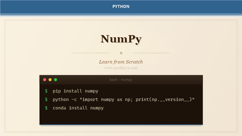
Before NumPy, doing linear algebra in Python meant nested lists and manual loops — painfully slow for anything beyond toy data. NumPy changed that by adding a homogeneous multidimensional array object that operates at C speed. I've used NumPy for everything from image processing (treating images as 3D arrays) to Monte Carlo simulations and signal processing. It's the foundation that Pandas, SciPy, scikit-learn, and TensorFlow all build on.
This tutorial focuses on the mental shift from Python lists to NumPy arrays. Once you internalize vectorized operations — operating on whole arrays without loops — you'll think about data manipulation differently. We'll cover array creation, indexing, broadcasting, linear algebra, and performance profiling.
Creating Arrays: The Core Data Structure
The ndarray (n-dimensional array) is homogeneous — all elements share the same type, stored in a contiguous memory block. This makes operations fast because the CPU can iterate cache-friendly memory. Create arrays from Python lists with np.array(), or use factory functions like np.zeros, np.ones, np.arange, and np.linspace for common patterns.
import numpy as np

zeros = np.zeros((3, 4))        # 3x4 matrix of 0.0
ones = np.ones((2, 3))          # 2x3 matrix of 1.0
sequence = np.arange(0, 10, 2)  # [0, 2, 4, 6, 8]
linear = np.linspace(0, 1, 5)   # [0.0, 0.25, 0.5, 0.75, 1.0]
random = np.random.randn(100)   # 100 normally distributed values
Indexing, Slicing, and Boolean Masks
NumPy indexing extends Python's slicing with multi-dimensional support. arr[i, j] indexes a 2D element, and arr[i:j, k:l] slices sub-arrays without copying data — views share the underlying buffer. Boolean masks are a superpower: passing a boolean array of the same shape selects elements where the mask is True, enabling vectorized conditional selection.
arr = np.arange(12).reshape(3, 4)
# array([[ 0,  1,  2,  3],
#        [ 4,  5,  6,  7],
#        [ 8,  9, 10, 11]])

print(arr[:, 1])      # Second column: [1, 5, 9]
print(arr[arr > 6])   # [ 7,  8,  9, 10, 11]

even = arr[arr % 2 == 0]
print(even)           # [ 0,  2,  4,  6,  8, 10]
Vectorized Operations and Broadcasting
Vectorized operations apply element-wise without explicit loops — the operation is pushed down to pre-compiled C code. Broadcasting extends this to arrays of different shapes: NumPy stretches the smaller array across the larger one as long as dimensions are compatible. This eliminates most loops in numerical code.
a = np.array([1, 2, 3])
b = np.array([10, 20, 30])
print(a + b)    # [11, 22, 33]
print(a * b)    # [10, 40, 90]

matrix = np.ones((3, 3))
row = np.array([1, 2, 3])
print(matrix + row)  # Broadcast row across all rows
Linear Algebra Operations
NumPy provides a full suite of linear algebra routines in np.linalg: matrix multiplication (dot or @), eigendecomposition, SVD, QR factorization, and solving linear systems. These call BLAS and LAPACK under the hood, the same libraries used by MATLAB and R, so performance is production-grade.
A = np.array([[3, 1], [1, 2]])
b = np.array([9, 8])

x = np.linalg.solve(A, b)          # Solve Ax = b => [2, 3]
eigvals, eigvecs = np.linalg.eig(A)
print(eigvals)                     # Eigenvalues

M = np.random.randn(5, 3)
U, S, Vt = np.linalg.svd(M)       # Singular value decomposition
Reshaping, Concatenation, and Aggregation
Reshaping changes an array's shape without copying data if possible (reshaping is a view when strides are compatible). Concatenation joins arrays along an axis, and aggregation functions like sum, mean, max, and std operate over entire arrays or along specific axes. The axis parameter determines which dimension to collapse.
data = np.random.randn(100, 5)
print(data.shape)            # (100, 5)

total_mean = data.mean()     # Scalar mean of all elements
col_means = data.mean(axis=0)  # Mean of each column
row_max = data.max(axis=1)   # Max of each row

stacked = np.vstack([data, data])  # Vertical stack: (200, 5)
Performance: Vectorization vs Loops
The performance gap between vectorized NumPy and pure Python loops is often 50-100x. The reason is twofold: CPython's loop overhead (type checking, reference counting) and cache locality (NumPy arrays are contiguous in memory). I always try to express operations as array expressions first, and only fall back to loops when the algorithm fundamentally requires it.
import time

n = 10_000_000
py_list = list(range(n))

# Pure Python
start = time.time()
result = [x**2 for x in py_list]
print("Python loop:", time.time() - start)

# NumPy vectorized
np_arr = np.arange(n)
start = time.time()
result = np_arr**2
print("NumPy:", time.time() - start)
Frequently Asked Questions
Why is NumPy faster than Python lists?
NumPy arrays store data in a contiguous C buffer with a fixed dtype, so element access doesn't involve Python object overhead. Vectorized operations loop in C, not Python, and leverage CPU SIMD instructions where possible.
Should I use np.array or np.matrix?
Use np.array. np.matrix is deprecated since it forces 2D and changes * behavior to matrix multiplication, which creates confusion. np.array's @ operator handles matrix multiplication explicitly.
How do I choose between NumPy and Pandas?
Use NumPy for pure numerical computation (linear algebra, random numbers, n-dimensional arrays). Use Pandas when you need labeled data, handling of missing values, or SQL-like groupby operations on heterogeneous columns.
What does 'copy=False' mean in array operations?
Many NumPy operations return views (no copy) when possible. A view shares memory with the original array, so modifying the view affects the original. If you need an independent copy, call .copy() explicitly.
Originally published on Ayodhyyya. Last updated June 1, 2026.